Pandas GroupBy Operations
Understanding GroupBy objects
import pandas as pd
titanic = pd.read_csv("titanic.csv")
titanic.head()
| survived | pclass | sex | age | sibsp | parch | fare | embarked | deck | |
|---|---|---|---|---|---|---|---|---|---|
| 0 | 0 | 3 | male | 22.0 | 1 | 0 | 7.2500 | S | NaN |
| 1 | 1 | 1 | female | 38.0 | 1 | 0 | 71.2833 | C | C |
| 2 | 1 | 3 | female | 26.0 | 0 | 0 | 7.9250 | S | NaN |
| 3 | 1 | 1 | female | 35.0 | 1 | 0 | 53.1000 | S | C |
| 4 | 0 | 3 | male | 35.0 | 0 | 0 | 8.0500 | S | NaN |
titanic.tail()
titanic.info()
<class 'pandas.core.frame.DataFrame'>
RangeIndex: 891 entries, 0 to 890
Data columns (total 9 columns):
 #   Column    Non-Null Count  Dtype
---  ------    --------------  -----
 0   survived  891 non-null    int64
 1   pclass    891 non-null    int64
 2   sex       891 non-null    object
 3   age       714 non-null    float64
 4   sibsp     891 non-null    int64
 5   parch     891 non-null    int64
 6   fare      891 non-null    float64
 7   embarked  889 non-null    object
 8   deck      203 non-null    object
dtypes: float64(2), int64(4), object(3)
memory usage: 62.8+ KB
titanic_slice = titanic.iloc[:10, [2,3]]
titanic_slice
| sex | age | |
|---|---|---|
| 0 | male | 22.0 |
| 1 | female | 38.0 |
| 2 | female | 26.0 |
| 3 | female | 35.0 |
| 4 | male | 35.0 |
| 5 | male | NaN |
| 6 | male | 54.0 |
| 7 | male | 2.0 |
| 8 | female | 27.0 |
| 9 | female | 14.0 |
titanic_slice.groupby("sex")
<pandas.core.groupby.generic.DataFrameGroupBy object at 0x0000027661634B20>
gbo = titanic_slice.groupby("sex")
type(gbo)
pandas.core.groupby.generic.DataFrameGroupBy
gbo.groups
{'female': [1, 2, 3, 8, 9], 'male': [0, 4, 5, 6, 7]}
l = list(gbo)
l
[('female',
        sex   age
  1  female  38.0
  2  female  26.0
  3  female  35.0
  8  female  27.0
  9  female  14.0),
 ('male',
      sex   age
  0  male  22.0
  4  male  35.0
  5  male   NaN
  6  male  54.0
  7  male   2.0)]
len(l)
2
l[0]
('female',
       sex   age
 1  female  38.0
 2  female  26.0
 3  female  35.0
 8  female  27.0
 9  female  14.0)
type(l[0])
tuple
l[0][0]
'female'
l[0][1]
| sex | age | |
|---|---|---|
| 1 | female | 38.0 |
| 2 | female | 26.0 |
| 3 | female | 35.0 |
| 8 | female | 27.0 |
| 9 | female | 14.0 |
type(l[0][1])
pandas.core.frame.DataFrame
l[1]
('male',
     sex   age
 0  male  22.0
 4  male  35.0
 5  male   NaN
 6  male  54.0
 7  male   2.0)
titanic_slice.loc[titanic_slice.sex == "female"]
| sex | age | |
|---|---|---|
| 1 | female | 38.0 |
| 2 | female | 26.0 |
| 3 | female | 35.0 |
| 8 | female | 27.0 |
| 9 | female | 14.0 |
titanic_slice_f = titanic_slice.loc[titanic_slice.sex == "female"]
titanic_slice_f
| sex | age | |
|---|---|---|
| 1 | female | 38.0 |
| 2 | female | 26.0 |
| 3 | female | 35.0 |
| 8 | female | 27.0 |
| 9 | female | 14.0 |
titanic_slice_m = titanic_slice.loc[titanic_slice.sex == "male"]
titanic_slice_m
| sex | age | |
|---|---|---|
| 0 | male | 22.0 |
| 4 | male | 35.0 |
| 5 | male | NaN |
| 6 | male | 54.0 |
| 7 | male | 2.0 |
titanic_slice_f.equals(l[0][1])
True
for element in gbo:
    print(element[1])
      sex   age
1  female  38.0
2  female  26.0
3  female  35.0
8  female  27.0
9  female  14.0
    sex   age
0  male  22.0
4  male  35.0
5  male   NaN
6  male  54.0
7  male   2.0
Splitting with many Keys
import pandas as pd
summer = pd.read_csv("datasets/summer.csv")
summer.head()
| Year | City | Sport | Discipline | Athlete | Country | Gender | Event | Medal | |
|---|---|---|---|---|---|---|---|---|---|
| 0 | 1896 | Athens | Aquatics | Swimming | HAJOS, Alfred | HUN | Men | 100M Freestyle | Gold |
| 1 | 1896 | Athens | Aquatics | Swimming | HERSCHMANN, Otto | AUT | Men | 100M Freestyle | Silver |
| 2 | 1896 | Athens | Aquatics | Swimming | DRIVAS, Dimitrios | GRE | Men | 100M Freestyle For Sailors | Bronze |
| 3 | 1896 | Athens | Aquatics | Swimming | MALOKINIS, Ioannis | GRE | Men | 100M Freestyle For Sailors | Gold |
| 4 | 1896 | Athens | Aquatics | Swimming | CHASAPIS, Spiridon | GRE | Men | 100M Freestyle For Sailors | Silver |
summer.info()
<class 'pandas.core.frame.DataFrame'>
RangeIndex: 31165 entries, 0 to 31164
Data columns (total 9 columns):
 #   Column      Non-Null Count  Dtype
---  ------      --------------  -----
 0   Year        31165 non-null  int64
 1   City        31165 non-null  object
 2   Sport       31165 non-null  object
 3   Discipline  31165 non-null  object
 4   Athlete     31165 non-null  object
 5   Country     31161 non-null  object
 6   Gender      31165 non-null  object
 7   Event       31165 non-null  object
 8   Medal       31165 non-null  object
dtypes: int64(1), object(8)
memory usage: 2.1+ MB
summer.Country.nunique()
147
split1 = summer.groupby("Country")
l = list(split1)
l[:2]
[('AFG',
         Year     City      Sport Discipline           Athlete Country Gender  \
  28965  2008  Beijing  Taekwondo  Taekwondo  NIKPAI, Rohullah     AFG    Men
  30929  2012   London  Taekwondo  Taekwondo  NIKPAI, Rohullah     AFG    Men

              Event   Medal
  28965     - 58 KG  Bronze
  30929  58 - 68 KG  Bronze  ),
 ('AHO',
         Year   City    Sport Discipline          Athlete Country Gender  \
  19323  1988  Seoul  Sailing    Sailing  BOERSMA, Jan D.     AHO    Men

                       Event   Medal
  19323  Board (Division Ii)  Silver  )]
len(l)
147
l[100][1]
| Year | City | Sport | Discipline | Athlete | Country | Gender | Event | Medal | |
|---|---|---|---|---|---|---|---|---|---|
| 5031 | 1928 | Amsterdam | Aquatics | Swimming | YLDEFONSO, Teofilo | PHI | Men | 200M Breaststroke | Bronze |
| 5741 | 1932 | Los Angeles | Aquatics | Swimming | YLDEFONSO, Teofilo | PHI | Men | 200M Breaststroke | Bronze |
| 5889 | 1932 | Los Angeles | Athletics | Athletics | TORIBIO, Simeon Galvez | PHI | Men | High Jump | Bronze |
| 5922 | 1932 | Los Angeles | Boxing | Boxing | VILLANUEVA, Jose | PHI | Men | 50.8 - 54KG (Bantamweight) | Bronze |
| 6447 | 1936 | Berlin | Athletics | Athletics | WHITE, Miguel S. | PHI | Men | 400M Hurdles | Bronze |
| 11005 | 1964 | Tokyo | Boxing | Boxing | VILLANUEVA, Anthony N. | PHI | Men | 54 - 57KG (Featherweight) | Silver |
| 18513 | 1988 | Seoul | Boxing | Boxing | SERANTES, Leopoldo | PHI | Men | - 48KG (Light-Flyweight) | Bronze |
| 20184 | 1992 | Barcelona | Boxing | Boxing | VELASCO, Roel | PHI | Men | - 48KG (Light-Flyweight) | Bronze |
| 21927 | 1996 | Atlanta | Boxing | Boxing | VELASCO, Mansueto | PHI | Men | - 48KG (Light-Flyweight) | Silver |
split2 = summer.groupby(by = ["Country", "Gender"])
l2 = list(split2)
l2[:2]
[(('AFG', 'Men'),
         Year     City      Sport Discipline           Athlete Country Gender  \
  28965  2008  Beijing  Taekwondo  Taekwondo  NIKPAI, Rohullah     AFG    Men
  30929  2012   London  Taekwondo  Taekwondo  NIKPAI, Rohullah     AFG    Men

              Event   Medal
  28965     - 58 KG  Bronze
  30929  58 - 68 KG  Bronze  ),
 (('AHO', 'Men'),
         Year   City    Sport Discipline          Athlete Country Gender  \
  19323  1988  Seoul  Sailing    Sailing  BOERSMA, Jan D.     AHO    Men

                       Event   Medal
  19323  Board (Division Ii)  Silver  )]
len(l2)
236
l2[104]
l2[104][0]
l2[104][1]
split-apply-combine explained
import pandas as pd
titanic = pd.read_csv("titanic.csv")
titanic_slice = titanic.iloc[:10, [2,3]]
titanic_slice
| sex | age | |
|---|---|---|
| 0 | male | 22.0 |
| 1 | female | 38.0 |
| 2 | female | 26.0 |
| 3 | female | 35.0 |
| 4 | male | 35.0 |
| 5 | male | NaN |
| 6 | male | 54.0 |
| 7 | male | 2.0 |
| 8 | female | 27.0 |
| 9 | female | 14.0 |
list(titanic_slice.groupby("sex"))[0][1]
| sex | age | |
|---|---|---|
| 1 | female | 38.0 |
| 2 | female | 26.0 |
| 3 | female | 35.0 |
| 8 | female | 27.0 |
| 9 | female | 14.0 |
list(titanic_slice.groupby("sex"))[1][1]
titanic_slice.groupby("sex").mean()
| age | |
|---|---|
| sex | |
| female | 28.00 |
| male | 28.25 |
titanic.groupby("sex").survived.sum()
sex
female    233
male      109
Name: survived, dtype: int64
titanic.groupby("sex")[["fare", "age"]].max()
| fare | age | |
|---|---|---|
| sex | ||
| female | 512.3292 | 63.0 |
| male | 512.3292 | 80.0 |
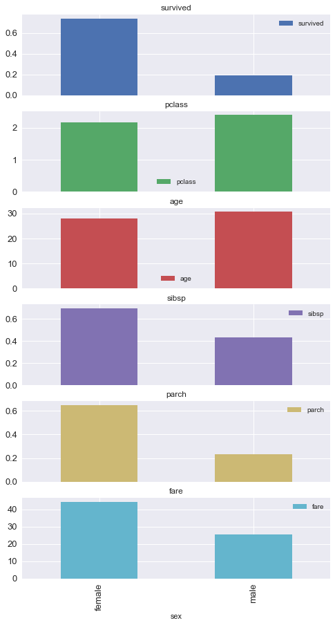
new_df = titanic.groupby("sex").mean()
new_df
| survived | pclass | age | sibsp | parch | fare | |
|---|---|---|---|---|---|---|
| sex | ||||||
| female | 0.742038 | 2.159236 | 27.915709 | 0.694268 | 0.649682 | 44.479818 |
| male | 0.188908 | 2.389948 | 30.726645 | 0.429809 | 0.235702 | 25.523893 |
%matplotlib inline
import matplotlib.pyplot as plt
plt.style.use("seaborn")
new_df.plot(kind = "bar", subplots = True, figsize = (8,15), fontsize = 13)
plt.show()
split-apply-combine applied
import pandas as pd
summer = pd.read_csv("summer.csv")
summer.head()
summer.info()
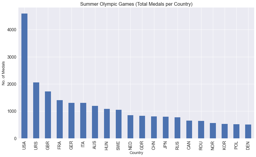
medals_per_country = summer.groupby("Country").Medal.count().nlargest(n = 20)
medals_per_country
Country
USA    4585
URS    2049
GBR    1720
FRA    1396
GER    1305
ITA    1296
AUS    1189
HUN    1079
SWE    1044
NED     851
GDR     825
CHN     807
JPN     788
RUS     768
CAN     649
ROU     640
NOR     554
KOR     529
POL     511
DEN     507
Name: Medal, dtype: int64
%matplotlib inline
import matplotlib.pyplot as plt
plt.style.use("seaborn")
medals_per_country.plot(kind = "bar", figsize = (14, 8), fontsize = 14)
plt.xlabel("Country", fontsize = 13)
plt.ylabel("No. of Medals", fontsize = 13)
plt.title("Summer Olympic Games (Total Medals per Country)", fontsize = 16)
plt.show()
titanic = pd.read_csv("titanic.csv")
titanic.head()
titanic.info()
titanic.describe()
titanic.fare.mean()
32.204207968574636
titanic.groupby("pclass").fare.mean()
pclass
1    84.154687
2    20.662183
3    13.675550
Name: fare, dtype: float64
titanic.survived.sum()
342
titanic.survived.mean()
0.3838383838383838
titanic.groupby("sex").survived.mean()
sex
female    0.742038
male      0.188908
Name: survived, dtype: float64
titanic.groupby("pclass").survived.mean()
pclass
1    0.629630
2    0.472826
3    0.242363
Name: survived, dtype: float64
titanic["ad_chi"] = "adult"
titanic.loc[titanic.age < 18, "ad_chi"] = "child"
titanic.head(20)
titanic.ad_chi.value_counts()
adult    778
child    113
Name: ad_chi, dtype: int64
titanic.groupby("ad_chi").survived.mean()
ad_chi
adult    0.361183
child    0.539823
Name: survived, dtype: float64
titanic.groupby(["sex", "ad_chi"]).survived.count()
sex     ad_chi
female  adult     259
        child      55
male    adult     519
        child      58
Name: survived, dtype: int64
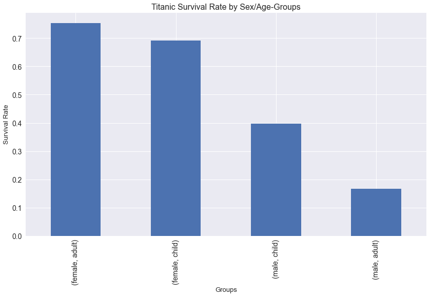
titanic.groupby(["sex", "ad_chi"]).survived.mean().sort_values(ascending = False)
sex     ad_chi
female  adult     0.752896
        child     0.690909
male    child     0.396552
        adult     0.165703
Name: survived, dtype: float64
w_and_c_first = titanic.groupby(["sex", "ad_chi"]).survived.mean().sort_values(ascending = False)
w_and_c_first.plot(kind = "bar", figsize = (14,8), fontsize = 14)
plt.xlabel("Groups", fontsize = 13)
plt.ylabel("Survival Rate", fontsize = 13)
plt.title("Titanic Survival Rate by Sex/Age-Groups", fontsize = 16)
plt.show()
Advanced Aggregation with agg()
import pandas as pd
titanic = pd.read_csv("titanic.csv", usecols = ["survived", "pclass", "sex", "age", "fare"])
titanic.head()
titanic.groupby("sex").mean()
| survived | pclass | age | fare | |
|---|---|---|---|---|
| sex | ||||
| female | 0.742038 | 2.159236 | 27.915709 | 44.479818 |
| male | 0.188908 | 2.389948 | 30.726645 | 25.523893 |
titanic.groupby("sex").sum()
| survived | pclass | age | fare | |
|---|---|---|---|---|
| sex | ||||
| female | 233 | 678 | 7286.00 | 13966.6628 |
| male | 109 | 1379 | 13919.17 | 14727.2865 |
titanic.groupby("sex").agg(["mean", "sum", "min", "max"])
| survived | pclass | age | fare | |||||||||||||
|---|---|---|---|---|---|---|---|---|---|---|---|---|---|---|---|---|
| mean | sum | min | max | mean | sum | min | max | mean | sum | min | max | mean | sum | min | max | |
| sex | ||||||||||||||||
| female | 0.742038 | 233 | 0 | 1 | 2.159236 | 678 | 1 | 3 | 27.915709 | 7286.00 | 0.75 | 63.0 | 44.479818 | 13966.6628 | 6.75 | 512.3292 |
| male | 0.188908 | 109 | 0 | 1 | 2.389948 | 1379 | 1 | 3 | 30.726645 | 13919.17 | 0.42 | 80.0 | 25.523893 | 14727.2865 | 0.00 | 512.3292 |
titanic.groupby("sex").agg({"survived": ["sum", "mean"], "pclass": "mean", "age": ["mean", "median"], "fare": "max"})
| survived | pclass | age | fare | |||
|---|---|---|---|---|---|---|
| sum | mean | mean | mean | median | max | |
| sex | ||||||
| female | 233 | 0.742038 | 2.159236 | 27.915709 | 27.0 | 512.3292 |
| male | 109 | 0.188908 | 2.389948 | 30.726645 | 29.0 | 512.3292 |
GroupBy Aggregation with Relabeling (new in Version 0.25)
import pandas as pd
titanic = pd.read_csv("titanic.csv", usecols = ["survived", "pclass", "sex", "age", "fare"])
titanic.head()
titanic.groupby("sex").survived.mean()
sex
female    0.742038
male      0.188908
Name: survived, dtype: float64
titanic.groupby("sex").agg(survival_rate = ("survived", "mean"))
| survival_rate | |
|---|---|
| sex | |
| female | 0.742038 |
| male | 0.188908 |
titanic.groupby("sex").agg({"survived": ["sum", "mean"], "age": ["mean"]})
| survived | age | ||
|---|---|---|---|
| sum | mean | mean | |
| sex | |||
| female | 233 | 0.742038 | 27.915709 |
| male | 109 | 0.188908 | 30.726645 |
titanic.groupby("sex").agg(survived_total = ("survived", "sum"),
                           survival_rate = ("survived", "mean"), mean_age = ("age", "mean"))
| survived_total | survival_rate | mean_age | |
|---|---|---|---|
| sex | |||
| female | 233 | 0.742038 | 27.915709 |
| male | 109 | 0.188908 | 30.726645 |
Transformation with transform()
import pandas as pd
titanic = pd.read_csv("titanic.csv")
titanic.head()
titanic.groupby(["sex", "pclass"]).survived.transform("mean")
0      0.135447
1      0.968085
2      0.500000
3      0.968085
4      0.135447
         ...
886    0.157407
887    0.968085
888    0.500000
889    0.368852
890    0.135447
Name: survived, Length: 891, dtype: float64
titanic["group_surv_rate"] = titanic.groupby(["sex", "pclass"]).survived.transform("mean")
titanic.head()
| survived | pclass | sex | age | sibsp | parch | fare | embarked | deck | group_surv_rate | |
|---|---|---|---|---|---|---|---|---|---|---|
| 0 | 0 | 3 | male | 22.0 | 1 | 0 | 7.2500 | S | NaN | 0.135447 |
| 1 | 1 | 1 | female | 38.0 | 1 | 0 | 71.2833 | C | C | 0.968085 |
| 2 | 1 | 3 | female | 26.0 | 0 | 0 | 7.9250 | S | NaN | 0.500000 |
| 3 | 1 | 1 | female | 35.0 | 1 | 0 | 53.1000 | S | C | 0.968085 |
| 4 | 0 | 3 | male | 35.0 | 0 | 0 | 8.0500 | S | NaN | 0.135447 |
titanic["outliers"] = abs(titanic.survived-titanic.group_surv_rate)
titanic[titanic.outliers > 0.85]
Replacing NA Values by group-specific Values
import pandas as pd
titanic = pd.read_csv("titanic.csv")
titanic.head(20)
titanic.info()
<class 'pandas.core.frame.DataFrame'>
RangeIndex: 891 entries, 0 to 890
Data columns (total 9 columns):
 #   Column    Non-Null Count  Dtype
---  ------    --------------  -----
 0   survived  891 non-null    int64
 1   pclass    891 non-null    int64
 2   sex       891 non-null    object
 3   age       714 non-null    float64
 4   sibsp     891 non-null    int64
 5   parch     891 non-null    int64
 6   fare      891 non-null    float64
 7   embarked  889 non-null    object
 8   deck      203 non-null    object
dtypes: float64(2), int64(4), object(3)
memory usage: 62.8+ KB
mean_age = titanic.age.mean()
mean_age
29.69911764705882
titanic.age.fillna(mean_age)
0      22.000000
1      38.000000
2      26.000000
3      35.000000
4      35.000000
         ...
886    27.000000
887    19.000000
888    29.699118
889    26.000000
890    32.000000
Name: age, Length: 891, dtype: float64
titanic.groupby(["sex", "pclass"]).age.mean()
sex     pclass
female  1         34.611765
        2         28.722973
        3         21.750000
male    1         41.281386
        2         30.740707
        3         26.507589
Name: age, dtype: float64
titanic["group_mean_age"] = titanic.groupby(["sex", "pclass"]).age.transform("mean")
titanic.head(20)
| survived | pclass | sex | age | sibsp | parch | fare | embarked | deck | group_mean_age | |
|---|---|---|---|---|---|---|---|---|---|---|
| 0 | 0 | 3 | male | 22.0 | 1 | 0 | 7.2500 | S | NaN | 26.507589 |
| 1 | 1 | 1 | female | 38.0 | 1 | 0 | 71.2833 | C | C | 34.611765 |
| 2 | 1 | 3 | female | 26.0 | 0 | 0 | 7.9250 | S | NaN | 21.750000 |
| 3 | 1 | 1 | female | 35.0 | 1 | 0 | 53.1000 | S | C | 34.611765 |
| 4 | 0 | 3 | male | 35.0 | 0 | 0 | 8.0500 | S | NaN | 26.507589 |
| 5 | 0 | 3 | male | NaN | 0 | 0 | 8.4583 | Q | NaN | 26.507589 |
| 6 | 0 | 1 | male | 54.0 | 0 | 0 | 51.8625 | S | E | 41.281386 |
| 7 | 0 | 3 | male | 2.0 | 3 | 1 | 21.0750 | S | NaN | 26.507589 |
| 8 | 1 | 3 | female | 27.0 | 0 | 2 | 11.1333 | S | NaN | 21.750000 |
| 9 | 1 | 2 | female | 14.0 | 1 | 0 | 30.0708 | C | NaN | 28.722973 |
| 10 | 1 | 3 | female | 4.0 | 1 | 1 | 16.7000 | S | G | 21.750000 |
| 11 | 1 | 1 | female | 58.0 | 0 | 0 | 26.5500 | S | C | 34.611765 |
| 12 | 0 | 3 | male | 20.0 | 0 | 0 | 8.0500 | S | NaN | 26.507589 |
| 13 | 0 | 3 | male | 39.0 | 1 | 5 | 31.2750 | S | NaN | 26.507589 |
| 14 | 0 | 3 | female | 14.0 | 0 | 0 | 7.8542 | S | NaN | 21.750000 |
| 15 | 1 | 2 | female | 55.0 | 0 | 0 | 16.0000 | S | NaN | 28.722973 |
| 16 | 0 | 3 | male | 2.0 | 4 | 1 | 29.1250 | Q | NaN | 26.507589 |
| 17 | 1 | 2 | male | NaN | 0 | 0 | 13.0000 | S | NaN | 30.740707 |
| 18 | 0 | 3 | female | 31.0 | 1 | 0 | 18.0000 | S | NaN | 21.750000 |
| 19 | 1 | 3 | female | NaN | 0 | 0 | 7.2250 | C | NaN | 21.750000 |
titanic.age.fillna(titanic.group_mean_age, inplace = True)
titanic.head(20)
| survived | pclass | sex | age | sibsp | parch | fare | embarked | deck | group_mean_age | |
|---|---|---|---|---|---|---|---|---|---|---|
| 0 | 0 | 3 | male | 22.000000 | 1 | 0 | 7.2500 | S | NaN | 26.507589 |
| 1 | 1 | 1 | female | 38.000000 | 1 | 0 | 71.2833 | C | C | 34.611765 |
| 2 | 1 | 3 | female | 26.000000 | 0 | 0 | 7.9250 | S | NaN | 21.750000 |
| 3 | 1 | 1 | female | 35.000000 | 1 | 0 | 53.1000 | S | C | 34.611765 |
| 4 | 0 | 3 | male | 35.000000 | 0 | 0 | 8.0500 | S | NaN | 26.507589 |
| 5 | 0 | 3 | male | 26.507589 | 0 | 0 | 8.4583 | Q | NaN | 26.507589 |
| 6 | 0 | 1 | male | 54.000000 | 0 | 0 | 51.8625 | S | E | 41.281386 |
| 7 | 0 | 3 | male | 2.000000 | 3 | 1 | 21.0750 | S | NaN | 26.507589 |
| 8 | 1 | 3 | female | 27.000000 | 0 | 2 | 11.1333 | S | NaN | 21.750000 |
| 9 | 1 | 2 | female | 14.000000 | 1 | 0 | 30.0708 | C | NaN | 28.722973 |
| 10 | 1 | 3 | female | 4.000000 | 1 | 1 | 16.7000 | S | G | 21.750000 |
| 11 | 1 | 1 | female | 58.000000 | 0 | 0 | 26.5500 | S | C | 34.611765 |
| 12 | 0 | 3 | male | 20.000000 | 0 | 0 | 8.0500 | S | NaN | 26.507589 |
| 13 | 0 | 3 | male | 39.000000 | 1 | 5 | 31.2750 | S | NaN | 26.507589 |
| 14 | 0 | 3 | female | 14.000000 | 0 | 0 | 7.8542 | S | NaN | 21.750000 |
| 15 | 1 | 2 | female | 55.000000 | 0 | 0 | 16.0000 | S | NaN | 28.722973 |
| 16 | 0 | 3 | male | 2.000000 | 4 | 1 | 29.1250 | Q | NaN | 26.507589 |
| 17 | 1 | 2 | male | 30.740707 | 0 | 0 | 13.0000 | S | NaN | 30.740707 |
| 18 | 0 | 3 | female | 31.000000 | 1 | 0 | 18.0000 | S | NaN | 21.750000 |
| 19 | 1 | 3 | female | 21.750000 | 0 | 0 | 7.2250 | C | NaN | 21.750000 |
titanic.info()
<class 'pandas.core.frame.DataFrame'>
RangeIndex: 891 entries, 0 to 890
Data columns (total 10 columns):
 #   Column          Non-Null Count  Dtype
---  ------          --------------  -----
 0   survived        891 non-null    int64
 1   pclass          891 non-null    int64
 2   sex             891 non-null    object
 3   age             891 non-null    float64
 4   sibsp           891 non-null    int64
 5   parch           891 non-null    int64
 6   fare            891 non-null    float64
 7   embarked        889 non-null    object
 8   deck            203 non-null    object
 9   group_mean_age  891 non-null    float64
dtypes: float64(3), int64(4), object(3)
memory usage: 69.7+ KB
Generalizing split-apply-combine with apply()
import pandas as pd
titanic = pd.read_csv("titanic.csv", usecols = ["survived", "pclass", "sex", "age", "fare"])
titanic.head()
titanic.groupby("sex").mean()
| survived | pclass | age | fare | |
|---|---|---|---|---|
| sex | ||||
| female | 0.742038 | 2.159236 | 27.915709 | 44.479818 |
| male | 0.188908 | 2.389948 | 30.726645 | 25.523893 |
female_group = list(titanic.groupby("sex"))[0][1]
female_group
| survived | pclass | sex | age | fare | |
|---|---|---|---|---|---|
| 1 | 1 | 1 | female | 38.0 | 71.2833 |
| 2 | 1 | 3 | female | 26.0 | 7.9250 |
| 3 | 1 | 1 | female | 35.0 | 53.1000 |
| 8 | 1 | 3 | female | 27.0 | 11.1333 |
| 9 | 1 | 2 | female | 14.0 | 30.0708 |
| ... | ... | ... | ... | ... | ... |
| 880 | 1 | 2 | female | 25.0 | 26.0000 |
| 882 | 0 | 3 | female | 22.0 | 10.5167 |
| 885 | 0 | 3 | female | 39.0 | 29.1250 |
| 887 | 1 | 1 | female | 19.0 | 30.0000 |
| 888 | 0 | 3 | female | NaN | 23.4500 |
314 rows × 5 columns
female_group.mean().astype("float")
C:\Users\LENOVO\AppData\Local\Temp/ipykernel_19564/2434558135.py:1: FutureWarning: Dropping of nuisance columns in DataFrame reductions (with 'numeric_only=None') is deprecated; in a future version this will raise TypeError.  Select only valid columns before calling the reduction.
  female_group.mean().astype("float")


survived     0.742038
pclass       2.159236
age         27.915709
fare        44.479818
dtype: float64
def group_mean(group):
    return group.mean()
group_mean(female_group)
C:\Users\LENOVO\AppData\Local\Temp/ipykernel_19564/359042690.py:2: FutureWarning: Dropping of nuisance columns in DataFrame reductions (with 'numeric_only=None') is deprecated; in a future version this will raise TypeError.  Select only valid columns before calling the reduction.
  return group.mean()


survived     0.742038
pclass       2.159236
age         27.915709
fare        44.479818
dtype: float64
titanic.groupby("sex").apply(group_mean)
C:\Users\LENOVO\AppData\Local\Temp/ipykernel_19564/359042690.py:2: FutureWarning: Dropping of nuisance columns in DataFrame reductions (with 'numeric_only=None') is deprecated; in a future version this will raise TypeError.  Select only valid columns before calling the reduction.
  return group.mean()
| survived | pclass | age | fare | |
|---|---|---|---|---|
| sex | ||||
| female | 0.742038 | 2.159236 | 27.915709 | 44.479818 |
| male | 0.188908 | 2.389948 | 30.726645 | 25.523893 |
titanic.nlargest(5, "age")
| survived | pclass | sex | age | fare | |
|---|---|---|---|---|---|
| 630 | 1 | 1 | male | 80.0 | 30.0000 |
| 851 | 0 | 3 | male | 74.0 | 7.7750 |
| 96 | 0 | 1 | male | 71.0 | 34.6542 |
| 493 | 0 | 1 | male | 71.0 | 49.5042 |
| 116 | 0 | 3 | male | 70.5 | 7.7500 |
def five_oldest_surv(group):
    return group[group.survived == 1].nlargest(5, "age")
titanic.groupby("sex").apply(five_oldest_surv)
Hierarchical Indexing (MultiIndex) with Groupby
import pandas as pd
titanic = pd.read_csv("titanic.csv", usecols = ["survived", "pclass", "sex", "age", "fare"])
titanic
summary = titanic.groupby(["sex", "pclass"]).mean()
summary
| survived | age | fare | ||
|---|---|---|---|---|
| sex | pclass | |||
| female | 1 | 0.968085 | 34.611765 | 106.125798 |
| 2 | 0.921053 | 28.722973 | 21.970121 | |
| 3 | 0.500000 | 21.750000 | 16.118810 | |
| male | 1 | 0.368852 | 41.281386 | 67.226127 |
| 2 | 0.157407 | 30.740707 | 19.741782 | |
| 3 | 0.135447 | 26.507589 | 12.661633 |
summary.index
MultiIndex([('female', 1),
            ('female', 2),
            ('female', 3),
            (  'male', 1),
            (  'male', 2),
            (  'male', 3)],
           names=['sex', 'pclass'])
summary.loc[("female", 2), :]
survived     0.921053
age         28.722973
fare        21.970121
Name: (female, 2), dtype: float64
summary.loc[("female", 2), "age"]
summary.swaplevel().sort_index()
| survived | age | fare | ||
|---|---|---|---|---|
| pclass | sex | |||
| 1 | female | 0.968085 | 34.611765 | 106.125798 |
| male | 0.368852 | 41.281386 | 67.226127 | |
| 2 | female | 0.921053 | 28.722973 | 21.970121 |
| male | 0.157407 | 30.740707 | 19.741782 | |
| 3 | female | 0.500000 | 21.750000 | 16.118810 |
| male | 0.135447 | 26.507589 | 12.661633 |
summary.reset_index()
| sex | pclass | survived | age | fare | |
|---|---|---|---|---|---|
| 0 | female | 1 | 0.968085 | 34.611765 | 106.125798 |
| 1 | female | 2 | 0.921053 | 28.722973 | 21.970121 |
| 2 | female | 3 | 0.500000 | 21.750000 | 16.118810 |
| 3 | male | 1 | 0.368852 | 41.281386 | 67.226127 |
| 4 | male | 2 | 0.157407 | 30.740707 | 19.741782 |
| 5 | male | 3 | 0.135447 | 26.507589 | 12.661633 |
stack() and unstack()
import pandas as pd
summer = pd.read_csv("summer.csv")
summer.head()
medals_by_country = summer.groupby(["Country", "Medal"]).Medal.count()
medals_by_country
Country  Medal
AFG      Bronze     2
AHO      Silver     1
ALG      Bronze     8
         Gold       5
         Silver     2
                   ..
ZIM      Gold      18
         Silver     4
ZZX      Bronze    10
         Gold      23
         Silver    15
Name: Medal, Length: 347, dtype: int64
medals_by_country.loc[("USA", "Gold")]
2235
medals_by_country.shape
(347,)
medals_by_country.unstack(level = -1)
| Medal | Bronze | Gold | Silver |
|---|---|---|---|
| Country | |||
| AFG | 2.0 | NaN | NaN |
| AHO | NaN | NaN | 1.0 |
| ALG | 8.0 | 5.0 | 2.0 |
| ANZ | 5.0 | 20.0 | 4.0 |
| ARG | 91.0 | 69.0 | 99.0 |
| ... | ... | ... | ... |
| VIE | NaN | NaN | 2.0 |
| YUG | 118.0 | 143.0 | 174.0 |
| ZAM | 1.0 | NaN | 1.0 |
| ZIM | 1.0 | 18.0 | 4.0 |
| ZZX | 10.0 | 23.0 | 15.0 |
147 rows × 3 columns
medals_by_country = medals_by_country.unstack(level = -1, fill_value= 0)
medals_by_country.head()
medals_by_country.shape
(147, 3)
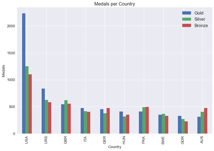
medals_by_country = medals_by_country[["Gold", "Silver", "Bronze"]]
medals_by_country.sort_values(by = ["Gold", "Silver", "Bronze"], ascending = [False, False, False], inplace = True)
medals_by_country.head(10)
| Medal | Gold | Silver | Bronze |
|---|---|---|---|
| Country | |||
| USA | 2235 | 1252 | 1098 |
| URS | 838 | 627 | 584 |
| GBR | 546 | 621 | 553 |
| ITA | 476 | 416 | 404 |
| GER | 452 | 378 | 475 |
| HUN | 412 | 316 | 351 |
| FRA | 408 | 491 | 497 |
| SWE | 349 | 367 | 328 |
| GDR | 329 | 271 | 225 |
| AUS | 312 | 405 | 472 |
import matplotlib.pyplot as plt
plt.style.use("seaborn")
medals_by_country.head(10).plot(kind = "bar", figsize = (12,8), fontsize = 13)
plt.xlabel("Country", fontsize = 13)
plt.ylabel("Medals", fontsize = 13)
plt.title("Medals per Country", fontsize = 16)
plt.legend(fontsize = 15)
plt.show()
medals_by_country.stack().unstack()
Country  Medal
USA      Gold      2235
         Silver    1252
         Bronze    1098
URS      Gold       838
         Silver     627
                   ...
NIG      Silver       0
         Bronze       1
TOG      Gold         0
         Silver       0
         Bronze       1
Length: 441, dtype: int64